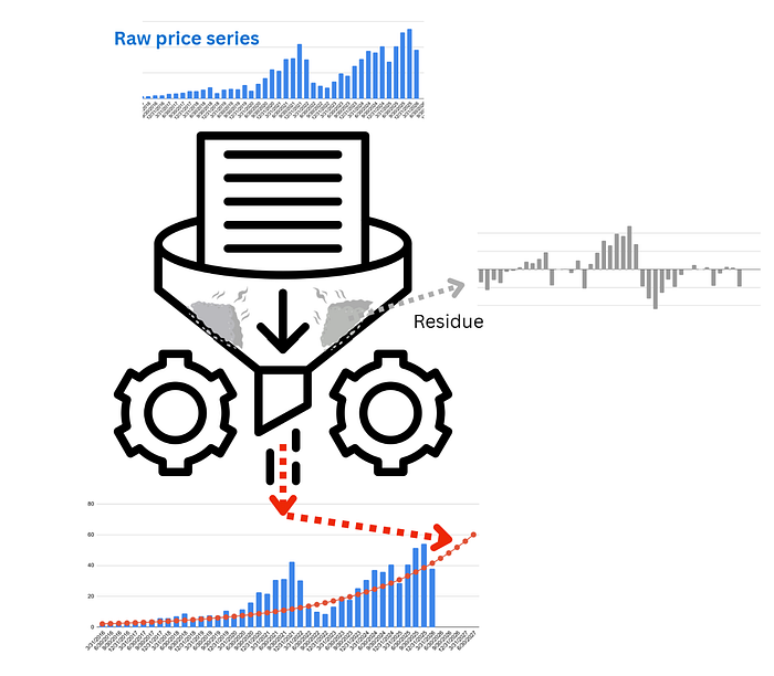
As soon as you draw such a line (the math is fairly straightforward), you come to grips with the next question, the more important one : How do you know your model of the markets is valid ? Why would you trust it.
So the question becomes : You fit a curve, through an index/ETF and called it a trend or ‘structure’. How do you know, its revealing genuine structure, or just a convenient narrative ?
In an earlier article, we saw how can a compounding curve be fitted to an ETF, to create a trendline of psychological reassurance. The assurance can really do wonders for your portfolio, by providing you a mental model of how should the portfolio look in 6 months and 6 years. This can really allow investors to sleep at night. But….
A fitted ETF growth curve is not merely a chart decoration. It is a hypothesis about the structure of returns.
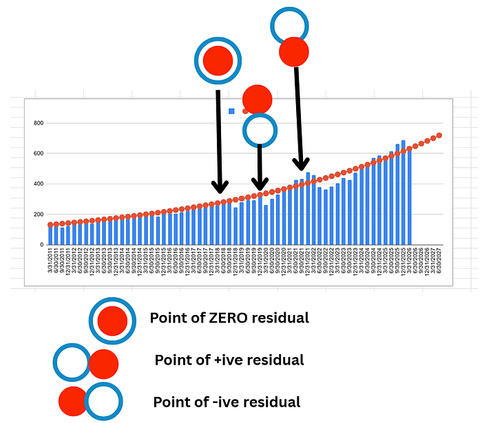
Because what you have in the form of a line, is actually a model. A model of the growth of something (a sector, a subsector within economy etc). When you have a model of a growth of a fund, like a NASDAQ index fund for example, you can check the model for future predictions about growth. The model can be made to predict any number of price points in the future. When you get a new (price) data point, you check it against the model. When the new data and the model agrees, you have no residual. Nothing left to ponder upon. But, — and that is where the fun begins — — when the model and the new price don't agree, you have a mismatch residual — a quantitatively non-zero signal that tells us of the price difference, that the model was unable to capture/predict successfully. The figure shows difference points on the curve with zero, -ive and +ive residuals.
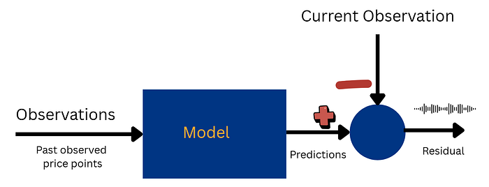
The idea is also shown diagrammatically as follows : A (chunk of past) price data going into the model to generate a prediction (of the current price), which can be tested against the current observation to yield the residual.
One might think that the modeled output, or prediction is the true output of the model — and it is to a large degree , but the success of the model, or a possible failure hidden underneath the model, lives deeper. It lives Inside the model residue.
You are (always) implicitly predicting
When you fit an exponential compounding line to the price data, it might seem a harmless annotation on the graph. It is anything but that.
By having that line, and showing it superimposed on the price chart, you are staking a claim — a hypothesis of sort, stated implicitly : that the prices have an underlying structure, represented by the red line.
What residuals actually mean
Technically a residual is :
the difference between the actual ETF path and the fitted compounding curve
but residuals are not just errors.
They are information about what the curve failed to explain.
If the residual still has structure, the model may be wrong or incomplete.
If the residual looks random and pattern-less, the fit may be credible. This means there was no more information inside the signal to be mined. So the residual is left with no information footprint.
A good fit does not erase all deviations. It leaves behind deviations that no longer seem systematic.
Hidden residual test
If we need to test, how our residual behaves, we need to subject the model to something fundamental. The technical name for it would be :
Parametric variations.
Put simply, it means that we tweak, or slightly disturb the parameters which define the model. We take the inferred parameters of the model, and disturb them every so slightly. For all disturbances, both positive and negative, we study the residual. If we can get a better looking residual after the disturbance, our parameter has found a new value, at its current value.
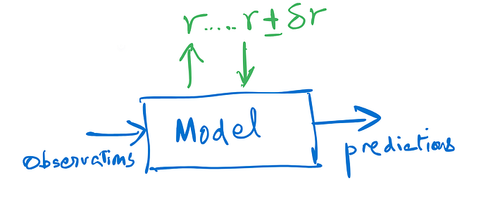
With this in mind, we first look at what happens with the statistically optimal rate. The inferred rate was 2.6% per quarter for the SPY index, representing S&P500. Here is a look at the residuals with the statistically optimal rate.
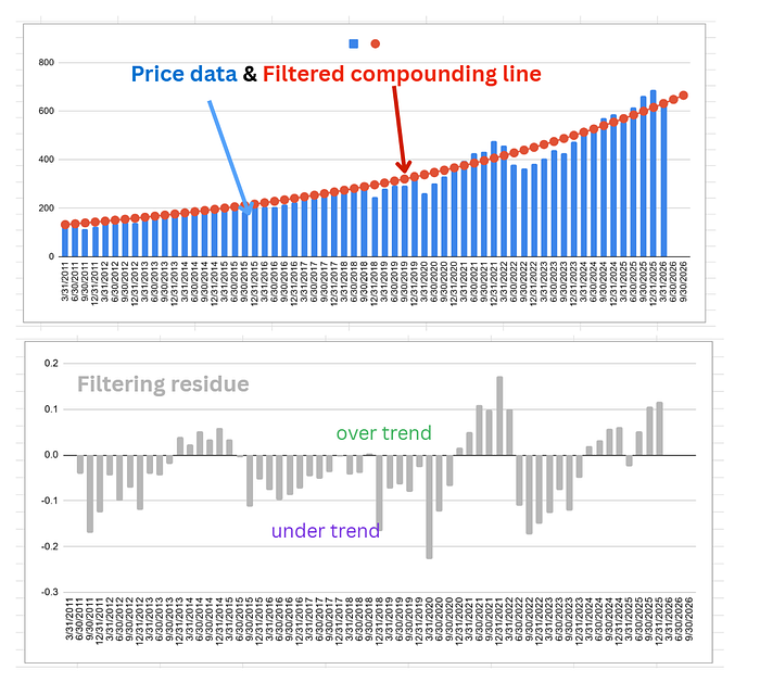
One can observe that residuals become positive and negative, and flip around the zero line, with seemingly even weightage, and no preference. It starts off negative, then flips positive, then stays negative for quite a while, and then has a positive->negative bout for several quarters.
Lets see what happens, when we use the rate of 2.4%, which is 0.2 percent below the optimal rate.
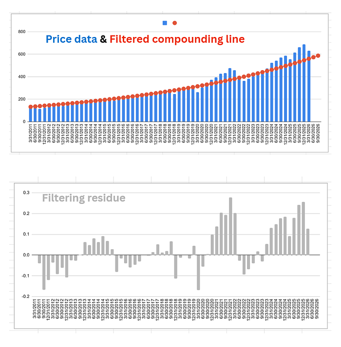
We see that while the earlier residuals flip between positive and negative, the later residuals have developed a bias towards a positive residual. The positive residuals signify that the curve is systematically underestimating growth.
Now a question might arise in the mind of the reader. What if I didnt have this later data available. What if I could only use the data until the year 2020. Here is a fit corresponding to that data
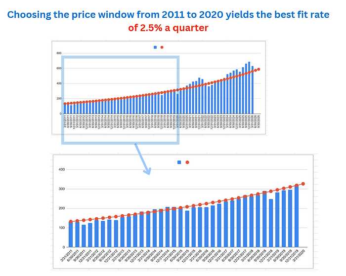
The best fit line now yields 2.5% a quarter, as opposed to 2.6% based on the earlier data. But this kind of variation is to expected around any statistically inferred number. The small variation is just a natural outcome of estimating a trend through some statistical method. The behavior of residuals still point you to an important fact : You are in the vicinity of the best rate.
Now lets look at a positive variation around the inferred rate. Instead of 2.6% a quarter, we can go to 2.8% to see what happens to the residuals.
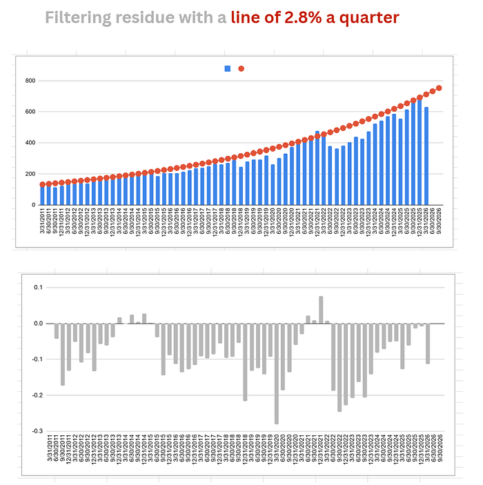
One can observe, the residue is now completely lopsided, with the red now perpetually overestimating the trend.
When you need assurance that the underlying structure of the signal has been captured, you need to look at the residual from the filtered trend. If the residuals fall on either side of the positive and negative, fairly evenly, you have found your structure, or very close to it. If you find them drifting to one side or the other, the fit needs to undergo more inspection. Either you need more data, for a better estimation of the model, or you need a better functional form for the model (like an exponential compounding function in our case). Here is the sequence :
- fit the “best” compounding rate
- then test slightly lower and slightly higher rates
- compare the residuals across these nearby fits
ask:
- does the chosen rate minimize systematic drift?
- do nearby rates introduce visible trend into the residual?
- does the optimum produce the most “noise-like” leftover pattern?
What this implies for investors and ETF holders
Our main goal here was to study, how can we think of the quality of the compounding curve.
When a compounding curve is inferred from real pricing data, its not as simple as just curve fitting.
You need to understand that the time interval taken into consideration has all kinds of scenarios baked in. And that the fitted curve represents a meaningful compounding lens to look at data.
The prescription here was to look at residuals. “Residuals” are a frequent occurance in data-science, statistics and machine learning tools. They can be thought of as hidden clues into the real-world implications of the model that is being inferred from the data. Once the residuals are examined, we learned that the distribution of residuals, i-e their drift up and down the zero line, offers a unique insight into whether the inferred model captures the pricing data. That is what makes the compounding curve, credible.
A credible compounding curve can help investors:
- understand whether current price is above or below trend
- judge the ETF’s historical growth character
- build more grounded expectations about future compounding
For the ETF analyzer I was building, I wanted the tool to do more than draw a trend line. I wanted it to test whether that trend line deserves to be trusted. And so I always display residuals. It gives a quick window into the behavior of the model.
Final Take away
The real test of a good ETF growth curve is whether the errors it leaves behind still whisper that something important has been missed.
A fitted CAGR becomes more believable when nearby growth rates fail in visible ways, and the chosen rate leaves the least structured residual behind.
And when that happens, we have an extremely valuable tool at hand, to determine the market undervaluation and overvaluation, and invest accordingly.